Warmup
Disclaimer: This week’s warmup has a lot of text. Don’t worry! There’s not that much actual work.
Part A: Musical Math
The main lab for this week involves audio processing. This exercise will cover some of the basics of how sound works in a computer.
Making Waves
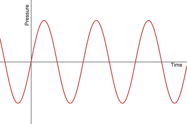
Sound is transmitted through air as a pressure wave, alternating regions of high- and low-pressure air, that cause our inner ears (and other things) to vibrate. The image you might have in your head of a “sound wave” is a graph of the air pressure hitting your eardrum over time. The peaks are high pressure, and the troughs are low pressure. We can model these pressure fluctuations with a sine wave, which is what we’ll be working with this week.
Choice of Waveforms
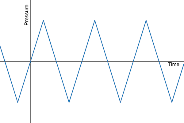
There are a number of different mathematical waveforms that we could use to model a sound wave. For example, we could use a triangle wave (shown below). Triangle waves have a sharp transition between the rising and falling portion of the wave. Such harsh changes in pressure are not often found in nature. This is one of the reasons we are choosing the gradually changing sine wave for our model.
There are two general principles that hold when dealing with sound waves.
- The higher the peaks and lower the troughs, the louder the sound.
- The closer together the peaks, the higher-pitched the sound.
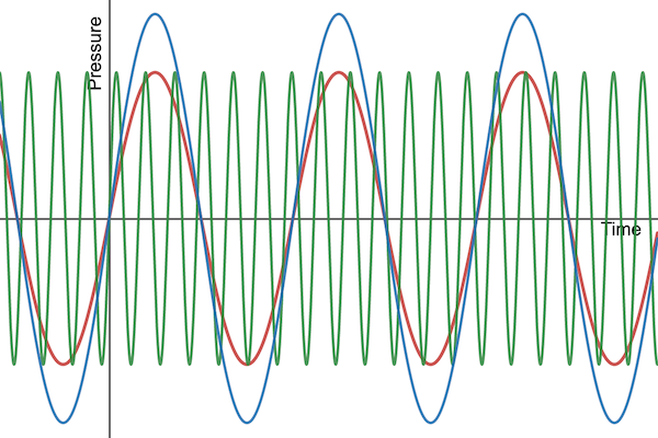
Let’s use the red sine wave from above as a reference. The blue sine wave below has higher amplitude (higher peaks and lower troughs), and will therefore produce a louder sound. The green sine wave, on the other hand, has the same amplitude but higher frequency (peaks are closer together). Therefore, the green sine wave with be the same volume but higher-pitched compared to the red sine wave.
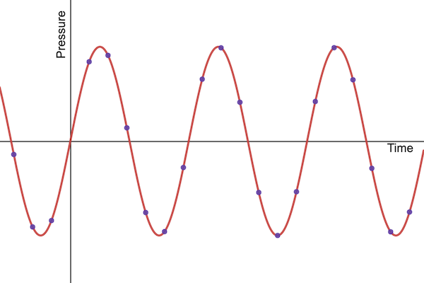
A real sound wave contains a lot of information. Every point in time is associated with a different air pressure. There are infinitely many such times, so how does a computer store all that information? It doesn’t. Instead, we use samples. Imagine just checking the value every 1/sample_rate seconds, where sample_rate is the number of samples you want to take each second. You would end up storing the values at certain points on the waveform (e.g., corresponding to the dots in the image below).
These values can be stored in a list. The benefit of modelling sound as a sine wave is that we have a function for the pressure over time (namely, the sine function), and so we can use that formula to compute the values of our samples. The value for the pressure at a given time $t$ is
$$ \mathrm{pressure}(t) = a \times \sin(2\pi \times f \times t) $$
where
- $t$ is the time measured in seconds,
- $a$ is the amplitude of the wave (higher = louder),
- $\sin()$ is the sine function,
- $\pi$ is the constant 3.14159, and
- $f$ is the frequency of the wave in cycles per second or Hertz (higher = higher-pitched).
If you want to use Python to generate a list of samples from a sine wave, just append each successive sample value to the list using the following formula:
samples.append(amp * math.sin(2 * math.pi * freq * i/sample_rate))
Here’s a breakdown of the formula’s new components:
samples[i]is a reference to theith element of thesampleslist,ampis the amplitude $a$,math.sin()is the sine function from themathmodule,math.piis Python’s stored value of the constant $\pi = 3.14156265…$,freqis the frequency $f$, andi/sample_rateis the calculation of time $t$ for samplei.
This formula aboves allows us to take a sample whenever the time is a multiple of 1/sample_rate.
Ok, so here’s the exercise. With your partner, use the formula for samples to compute the first 10 samples (i.e., i=0,...,9) when amp=1, freq=1, and sample_rate=10. You can use the console to do the computation. If you have a convenient way of plotting them, even better! You should see how they form the general shape of a wave.
Pitch
You won’t just be making sound in this lab, you’ll be making music. The Western scale has 12 notes, which repeat as you go up in pitch. Each corresponds to a key on the piano keyboard. After 12 notes (somewhat unhelpfully called half tones), you’ve traveled an octave, after which point you’ll hear the same notes as before, but higher in pitch. Here’s the weird thing: when you go up 12 notes, the frequency doubles. In general, what you see as linear progress up a keyboard is actually a multiplicative change in frequency. Since an octave is divided into 12 half tones, the doubling of frequency is divided up across the 12 tones as well. In other words, increasing the frequency by 1 half tone increases the frequency by a factor of 2**(1/12) (i.e., $\sqrt[12]{2}$).
Here are some examples to illustrate the discussion above.
- The A note that orchestras usually tune to has a frequency of 440Hz.
- The A an octave below that has a frequency of 220Hz (this note is called A220).
- The note one half tone above A220, an A#, has a frequency of
220*(2**(1/12)). - The C between A220 and A440 is sometimes called “Middle C”. It’s 3 half tones above A220 and has a frequency of
220*(2**(1/12))*(2**(1/12))*(2**(1/12))which is more concisely written as220*(2**(3/12)).
Here’s a quick exercise for you to check your understanding.
- What’s the frequency of the note an octave above A440 (A)?
- What’s the frequency of the note 5 half tones above A440 (D)?
- What’s the frequency of the note 2 half tones below A440 (G)?
Note that the letter names aren’t important for getting the right answer. They’re just there in case you’re curious about note names.
Part B: Opinion Dynamics
The Problem
In this exercise, you’ll see a couple of the most common object-oriented programming bugs and get practice testing object-oriented programs. In the process, you’ll do some computational social science—the code for this exercise models opinions spreading on social networks. Here’s the story you should have in mind: you’ve got a population of people, and each person starts with an initial opinion, which is a number between 0 and 1. Think of 0 as representing “I hate board games,” and 1 being “I love board games.” With something like that, it’s reasonable to expect people to be influenced over time by their friends’ opinions. The code here will crudely model this phenomenon.
We’ll model our simple social network in the following way: each person will be a node, and they’ll have links pointing to the people they like. For example, you might have the following:
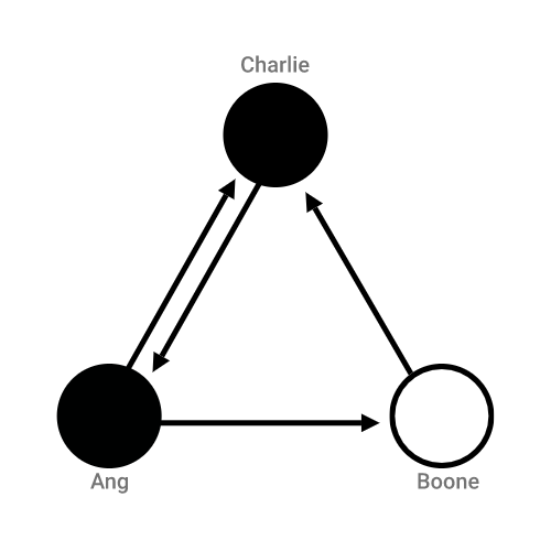
Each person’s node is colored in proportional to their initial opinion: 0 is black, 1 is white, and in-between values would be gray. Note that it’s possible to like someone who doesn’t like you. Ang likes Boone, but Boone does not like Ang.
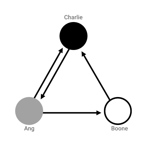
Here’s how we’ll capture opinion dynamics in a step-by-step method. Each step, we’ll pick someone at random from the population. That person will then update their opinion by taking the average opinion of all the people they like, including themselves. In our example, if we chose Ang to update, their opinion would go from 0 to 0.33, because among the people they like, two people hate board games (themselves and Charlie), and one person loves board games (Boone). In the updated graph below, Ang’s shade got a bit lighter.
If you update lots of times, you might hope the network will settle on a steady-state opinion, and that this opinion will depend on the network structure. Pretty cool! If you want, take a moment with your partner to discuss how you might set up such a simulation.
The Program
We have started implementing the Person class and some test code in opinion.py – it is set up to do the simulation as described above. Like many files which define and then test/use a class, we have the class definition at the top of the file and the main() function at the bottom. Your goal is to (a) debug some of the class methods and (b) test the simulation by adding and running code in main().
Start by taking a look at the Person class and then perform the following steps. Note that update() is broken and you’ll resolve that as the second step:
- Add code to
main()that will help you eventually test theupdate()method. Think about what the simplest example of updating might be. We suggest making 2Personinstances, one who likes video games and one who does not, and having one befriend the other. This is like having a network with two people and one arrow connection. If you follow these instructions, once you runupdate(), the befriended friend should have an opinion of 0.5. - You need to debug
update()prior to testing it. The issue is thatupdate()is missing fourself.references. Figure out where they go, add them to the code, and use the test from above to check you fixed all the errors.
Now let’s test the whole simuation! To do so, execute the following steps:
- Read over the code in
main()that runs the functionupdate_step(), which picks a person and asks them to update. Spend some time trying to figure out what the test code does. update_step()is currently broken. Use the test code to help you fix the bug inupdate_step().
Extra
Now that you’ve got working code, play with it some! Here are some questions you could ask. You can use the debugging code as starter code, but modify it to perform a few experiments. You don’t need complete answers to these questions, but you and your partner should try and come up with some guesses.
- If you call
update_step()enough times, do opinions always converge to a common value? How many steps does it take? - If you rerun the code twice, do the opinions converge to the same value?
- How do the final opinions depend on who is friends with whom?
- How would you add to this model to make it more realistic?